

When it comes to important processes like annual reviews, goal-setting and compensation reviews, your HR team most likely does a lot of the heavy lifting. Given just how important these processes are, that is no small feat.
The Complete Guide to Compensation Reviews in Microsoft Excel
You don’t have to involve your full finance team or be a spreadsheet guru to create a comp review. With just Excel and the steps in this guide, you can create a great comp review to retain top talent and keep costs in check. Wondering where to start? Related resource Compensation Planning: what it is and why you need it.
Make sure to download a copy of the salary benchmark Excel spreadsheet, which you’ll be able to use with your own data to create a comp review, rapidly.
How to Set Up Your Data For An Excel Compensation Review
When you build an Excel spreadsheet, the most important part is how you set the data structure. With the proper data structure, all of your analysis work is easier.
As you start to prepare your comp review, here’s a guide to the fields you should capture:
- Employee name – all of your data should be captured at an “employee level”, meaning it’s specific to each employee. You’ll need to capture the first and last name for each employee in separate columns, each on their own row.
- Current base salary – the current base salary is the starting point for all analysis, so make sure that you have this for each employee.
- Department (function) – comp structures vary by job role and function. Make sure to log the department for each employee so that you can apply comparisons accurately.
- Title – remember, the goal is to compare individuals to the overall population to find outliers. List the title for each employee so that you can make proper comparisons.
- Last year’s comp increase – every company goes through lean years. Sometimes, you’ll need to curtail raises so that you can make your budget goals. But make sure you track those adjustments each year so that employees aren’t disappointed in multiple years.
- Location – distributed teams are more popular than ever, so it’s important to note where each employee is working. Make sure to account for the cost of living for each employee based on location.
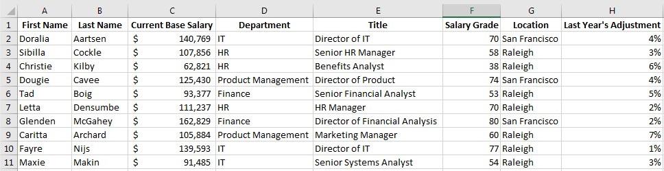
I call this tab the Base Data. It’s the single source of all your current information. Capture the data with care so that all of your analysis work is accurate.
After you capture your data in an Excel spreadsheet, you’re ready to start analyzing it. That means reviewing and summarizing. Let’s learn more about summarizing data for your comp review.
How to Create a Salary Benchmark in Microsoft Excel
When you review compensation, it helps to compare individuals to the overall population. Compensation reviews are designed to identify outliers so that you can adjust their compensation accordingly.
The first step is to create a salary benchmark. This helps you organize and summarize your data so that you can review situations that need to be adjusted.
Your data is already captured for each employee, so how do you find meaning in it? The answer is to summarize it and create averages and other data points. These are used to compare current salary to others.
With the help of an Excel pivot table, we can take our comp data and summarize it. Then, we can compare individuals to the overall population. Highlight columns A – H, then go to the Insert > PivotTable option on Excel’s ribbon.
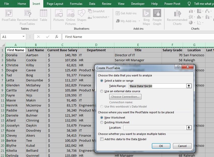
On the pop-up menu, make sure you leave the option set to Select a table or range and have all of your data highlighted. It should include all columns from A to H for our example. Then, click OK to create a pivot on a new sheet. You’ll see a new report builder appear.
Pivot tables are used to summarize data. I think of them as powerful, drag-and-drop reports. In our example, we’ll want to create three key data points for a salary benchmark:
- The average for each job title
- The maximum pay for each job title
- The minimum pay for each job title
Notice that we want to divide our data by department and job title. In our example, we need to put each division and title on its own row.
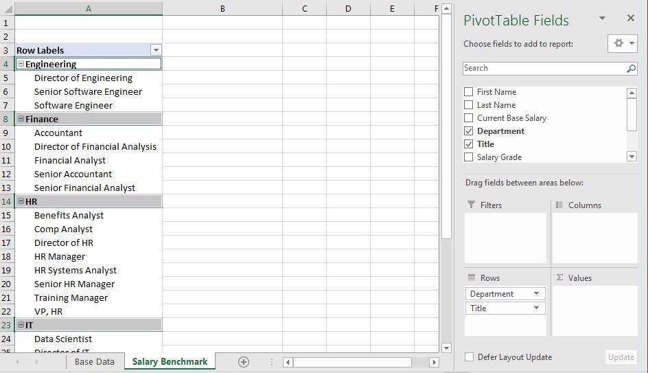
On the PivotTable Fields option, click and drag Department to the Rows section below. You’ll see each department in your data appear on its own row. Then, drag-and-drop Title underneath Department. Now, your pivot will match mine in the screenshot above, with each title on its own row.
So far, we’ve listed the job titles and departments. But what we really need are numeric values for the salary. This creates a benchmark.
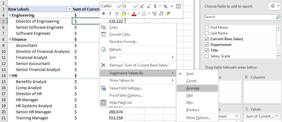
Drag and drop the Current Base Salary field into the Values box on the PivotTable builder. You’ll see a new column called Sum of Current Base Salary pop into the PivotTable. This field sums up the salaries paid for each job title.
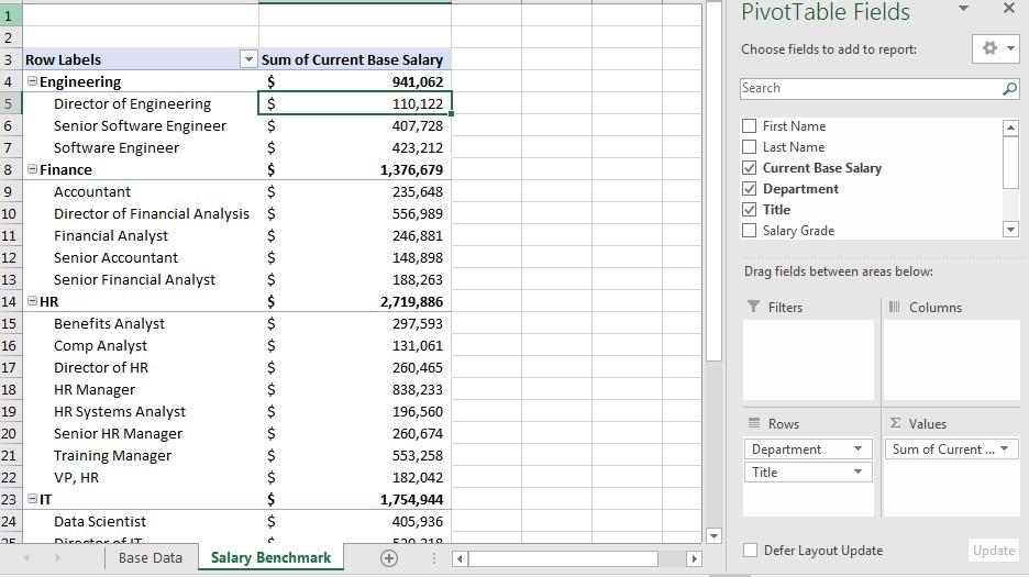
But what we really need is the Average. The sum of salaries doesn’t really tell us anything about our data. Right-click on the amounts and choose Summarize Values By > Average to change these to the average.
You’ve created an average for each job title. Now, drag Current Base Salary into the Values box two more times. Then, right-click on the new columns and choose Summarize Values By > Max and Min for the two new columns.
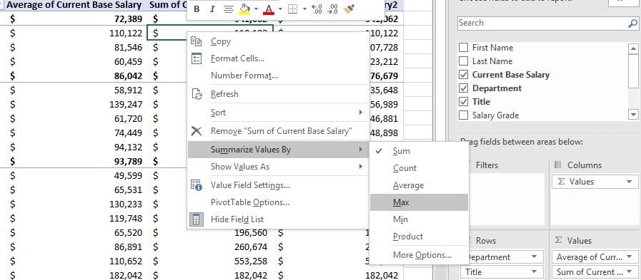
That’s it! You’ve created an average, max, and minimum salary for each job title in your organization. These data points are really helpful as you create your compensation adjustments.
How to Compare Employee Salaries to Peers
With our salary benchmark, we’ve created a useful guide to average salaries, plus high and low points on the curve. Now, it’s time to take those data points and compare each individual salary accordingly.
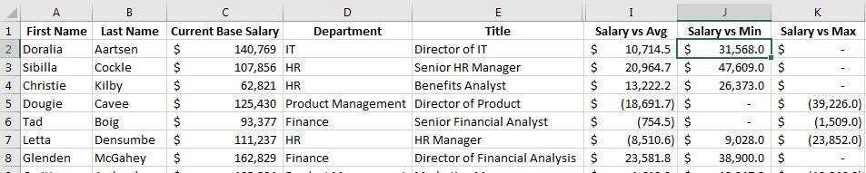
Back in our Base Data tab, let’s create several new columns:
- Salary vs Avg
- Salary vs Min
- Salary vs Max
Now, let’s pull those data points from our benchmark. Starting in the Salary vs Avg column, let’s write a VLOOKUP. This formula will use each title’s average, max and minimum salaries. In Column I, let’s write this formula:
=VLOOKUP(E2,‘Salary Benchmark’!A:D,2,FALSE)
This formula grabs the job title from cell E2, then matches it to a title in “Salary Benchmark” and shows the average for each title.
Now, we’ll write a formula to subtract an individual employee’s salary versus the average:
=C2-VLOOKUP(E2,‘Salary Benchmark’!A:D,2,FALSE)
Let’s write two more formulas in columns J and K respectively. You can use the same formula and change only one part, the column to match from the Benchmark tab. Change “2” to “3” for the minimum, and “3” to “4” for the maximum.
=C2-VLOOKUP(E2,‘Salary Benchmark’!A:D,3,FALSE)
=C2-VLOOKUP(E2,‘Salary Benchmark’!A:D,4,FALSE)
Pull each of these formulas all the way down the column to extend them and create comparisons for each and every employee. This creates comparisons for each salary versus the average, maximum, and minimum points.
Her’s what a “0” means for each of these fields:
- If the Average column shows a 0, it indicates the employee makes exactly the average salary for their title.
- If the Minimum column shows a 0, it indicates the employee makes the minimum for their title.
- If the Maximum column shows a 0, it indicates the employee makes the maximum for their title.
Comparison to Market
Performing a comparison to the market is a crucial step to help you retain your employees. Without measuring your salary versus the market, you risk losing your top employees.
Here’s what you need to do:
- Create a list of all the titles in your organization that you need to find comparable salaries for
- Get data on salaries from competing sources.
- Match up the titles in your competing data
The hardest part of creating a comparison to market is getting Here are a few ideas for sources on compensation data:
- Use LinkedIn and Glassdoor data to build up your own compensation survey.
- Source salary data from a reliable service like SHRM Compensation Data Center.
- Ask employees for compensation data when they accept counteroffers.
Create a new tab in your workbook called Competitor Salaries, and let’s copy and paste the entire column from our Base Data tab that includes job titles. Then, highlight the column and choose Data > Remove Duplicates on Excel’s ribbon.
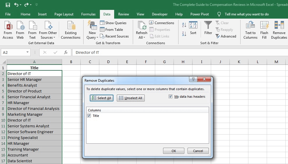
This creates exactly one instance of each job title.
Now, in column B, start listing your competitor job titles and match them up. Create a list of corresponding job titles along with competitor salaries.
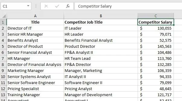
We have everything we need to benchmark our data versus the competition now. Let’s jump back to the Base Data tab. In a new column titled, Salary vs Competitor, just add this formula to complete your comparison:
=VLOOKUP(E2,’Competitor Salaries’!A:C,3,FALSE)
Cost of Living And Other Factors
The cost of living is a real drag on raises. Getting a 1% raise is a slap in the face as consumers catch the cost of living rise by 2% in many economies. Of course, you’re managing your payroll costs with budgets in mind, but so are employees in their households!
One popular way to monitor inflation is with the CPI, or consumer price index. It’s calculated and updated by the Bureau of Labor Statistics. It focuses on costs and provides a good guidepost to monitor rising costs.
Other factors might include monitoring high potential employees or high-need areas of your company. These go beyond the numbers and help you keep key positions staffed.
Applying Compensation Adjustments
All of the data above supports a compensation review. It gives you the points you need to make adjustments. Work with your managers and teams to determine which employees need adjustment, and how much that should be.
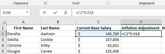
Let’s create a new sheet in our workbook to apply our compensation adjustments. Let’s call it Salary Adjustments. It helps to create a standalone sheet for this so that you can share it with your managers and employees when finished – cleanly.
Let’s create salary adjustments in two columns:
- Inflation adjustment – capturing an “across-the-board” adjustment
- Merit adjustment – add an employee-specific adjustment with individual adjustments
Then, we’ll sum it up in a column called Total Adjustment.
In the Inflation adjustment column, multiply the base salary times your agreed-upon inflation adjustment. I’ll apply a 1.8% increase across the board, and pull the formula down to calculate it for each employee.
Now, let’s create a merit adjustment in column E. Multiply base salary times the individual adjustment percentage to create the merit-based adjustment.
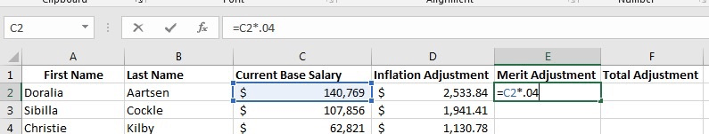
Finally, create a sum in Column F for D and E. You’ve calculated your total adjustment, and now you’re ready to share!
5 Key Takeaways To Perform Your Comp Review
Once you structure your data properly, just follow the steps in this tutorial to create a compensation review in Excel. You’ll have everything you need to adjust salaries so that you never lose top talent.
Remember these 5 points as you launch your comp review:
- Make sure that you prioritize the steps to create your salary benchmark. Knowing your current salaries and comparing them with others is the key to a successful comp review.
- Don’t miss out on comparing comp to the competition. You’ll reduce the risk of losing talent to others in your area and industry.
- Don’t forget about factors “outside the numbers.” Paying top talent above-market is a great example.
- Separate your merit and cost of living adjustments. This helps drive better conversations with your leadership.
- The approach in this tutorial is a great way to review comp, but there are always many factors to balance. Work with management and your managers to ensure that your increases fit budget and performance targets.